Traffic Sign Recognition

Summary

In this project, a classifier to recognize traffic sign was built based on Convolutional Neural Networks, which is a project of the Udacity Self-driving Cars Nanodegree program. The model was trained on a fraction of the German Traffic Sign dataset, which is provided as pickled files by the Self-driving car program. The final validation accuracy of our model was 97%, and the test accuracy was 98%. Six images downloaded from the internet were also used to test the model, and a accuracy of 66.7% was achieved.

The document includes following sections

Data set summary and exploration
Data augmentation and preprocessing
Model architecture design
Make prediction on new images
Softmax probabilities of the new images
Visualize feature maps of convolutional layers

Data Set Summary & Exploration

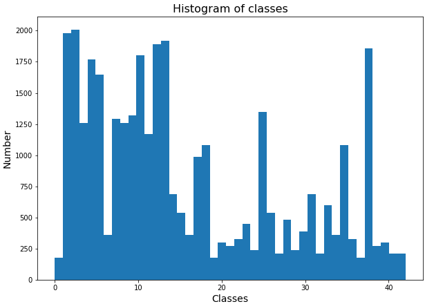
The provided dataset was explored with Pandas. Images of the dataset have been resized to 32x32, and all of them are RGB color images. There are 34799 training images, 12630 validation validation images, and 4410 test images. There are 43 unique categories of traffic signs in the data. Below is the histogram showing size of each category in the training data, which indicates that the dataset is asymmetric. Some categories have more than 1000 examples, while others have less than 200 examples.

alt text

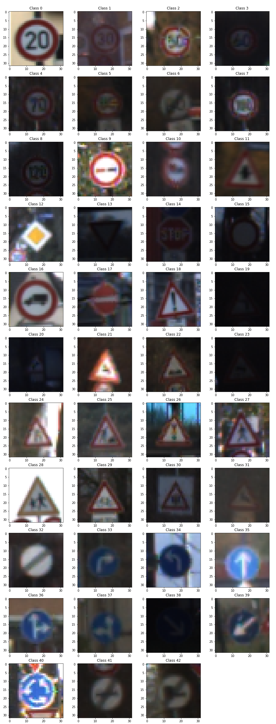
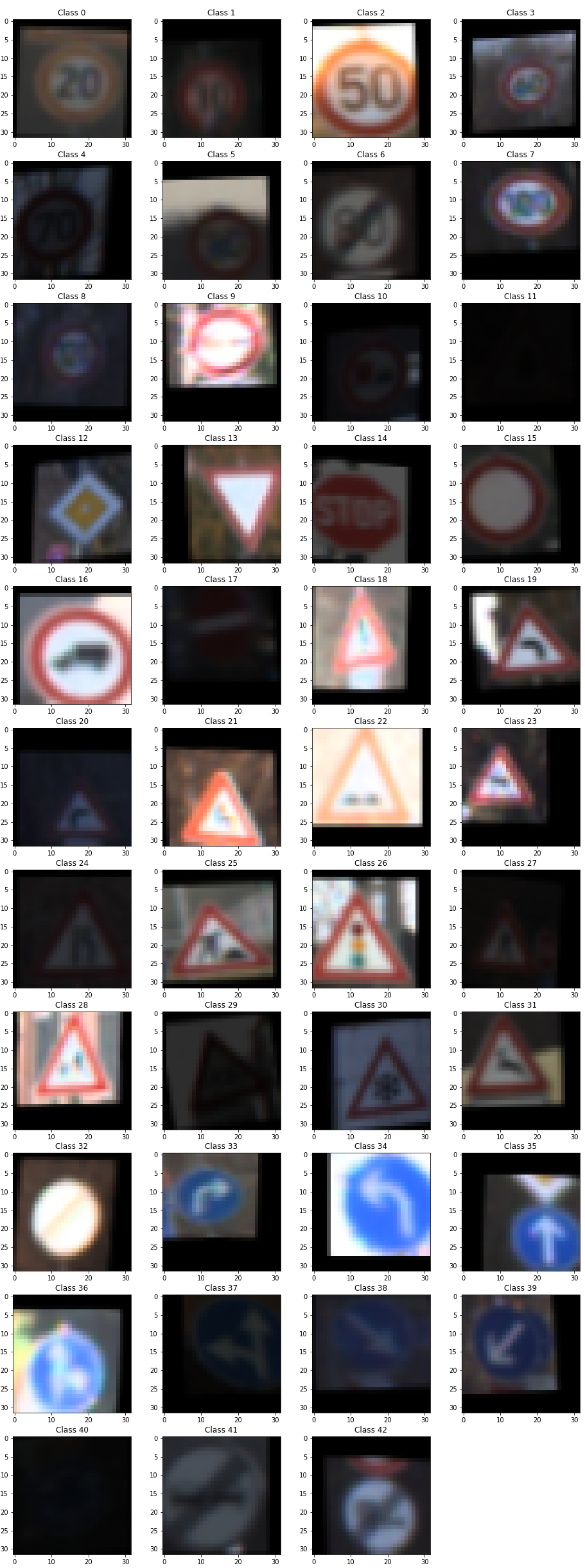
43 images was shown below with one arbitrary image from each category of the training image. The traffic signs in the train image have been pruned such that they are ovarally in similar size and in the center of the images. However, the intensity significantly varies from images to images, and some images were not taken precisely in the front view and some were not exactly aligned perpenticular to the ground.

Data Augmentation and Preprocessing

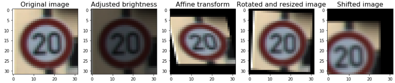
Since the dataset is asymmetric and the size of each category is not sufficient for a complex ConvNet mode, data augmentation is required for this dataset to avoid overfitting of our model, and the augmentation can be completed by vertically and horizontally shifting, resizing, warping, and changing brightness of original training images with given parameter. Examples of shifting, resizing, image warping, changing brightness are shown below with the 20km speed limit sign.

My assumption is that the training data set reflects road conditions, and the road condition determines that certain traffic signs are met more frequently than others. Hence, the proportion of categories is maintained in my augmented data. The size of a categoriy in the augmented data is 7 times more than the size of the same category in the original data. For each categary, my function randomly picks an image from the original data, on which a random combination of changing brightness, horizontal and vertical shifting, rotation and resizing, and affine transform will be applied. Examples of images of augmentated data are plotted below.

Preprocessing is also required for images to be input to the neural network. The basic step is normalization. Other techniques, such as converting the original RGB images to grayscale or applying histogram equalization to images, have also been tested. However, no significant improvement has been observed with grascale or histogram equalized images. Thus, simple normalization is the only preprocessing applied in this study. The performance of my final model is obtained from image augmentation and the network architecture.

Model Architecture Design

The layer pattern of my ConvNet model is as follows

Layer	Description
Input	32x32x3 RGB image
Convolution 3x3	1x1 stride, same padding, outputs 32x32x16
RELU
DROPOUT
Convolution 3x3	1x1 stride, same padding, outputs 32x32x32
RELU
Max pooling	2x2 stride, outputs 16x16x32
DROPOUT
Convolution 3x3	1x1 stride, same padding, outputs 16x16x64
RELU
DROPOUT
Convolution 3x3	1x1 stride, same padding, outputs 16x16x64
RELU
Max pooling	2x2 stride, outputs 8x8x64
DROPOUT
Convolution 3x3	1x1 stride, same padding, outputs 8x8x128
RELU
DROPOUT
Convolution 3x3	1x1 stride, same padding, outputs 8x8x128
RELU
Max pooling	2x2 stride, outputs 4x4x64
DROPOUT
Fully connected	2048x2048
DROPOUT
Fully connected	2048x1024
DROPOUT
Fully connected	1024x10

The model includes six convolutional layers and three fully connected layers. Connected convolutional layers enables a wide view on the inputs for the model. Every convolutional layer and fully connected layer is followed by a dropout layer, which has effectively reduced overfitting. A pooling layer is used after every two convolutional layers, hence the size of feature maps are not shrinking too fast.

The Adam optimizer was used to train this model. The learning rate is 2e-4 and the dropout probability is 0.5. A minibatch size of 128 is chosen for this model. The model achieves 97% validation accuracy in 70 epochs. The ccuracy on the pickled test data is 98%.

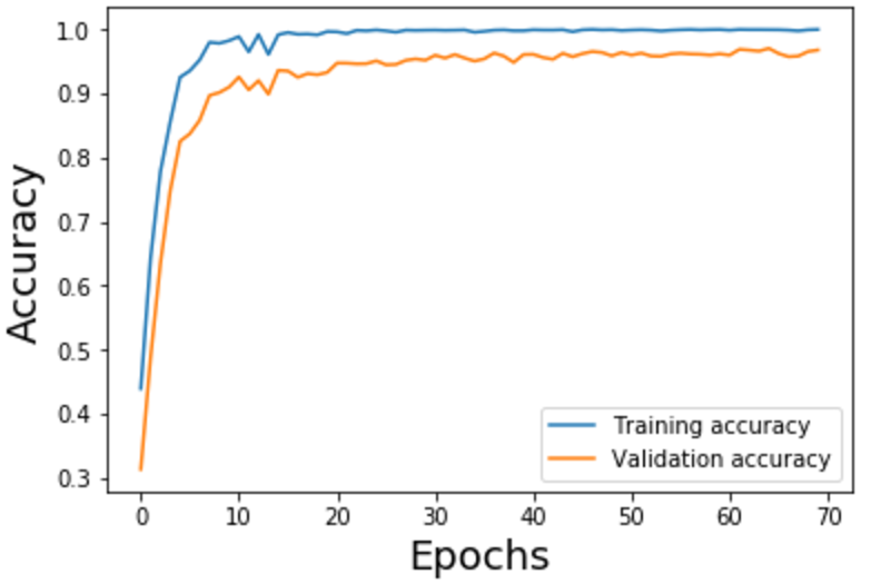
I started the architecture design with LeNet, because it is the very first successful ConvNet for image classification. I have achieved 89-91% validation accuracy with LeNet on the original training data. At the moment, the training accuracy quickly converged to 100%, which indicates overfitting. My first improvement was testing dropout layers at different depth of LeNet, which ends up with a dropout layer following every other layers. This improvement quickly help my model achieve 93-94% accuracy. Then with two more convolutional layers and image augmentation, I finalized my model to the current architecture.

Test a Model on New Images

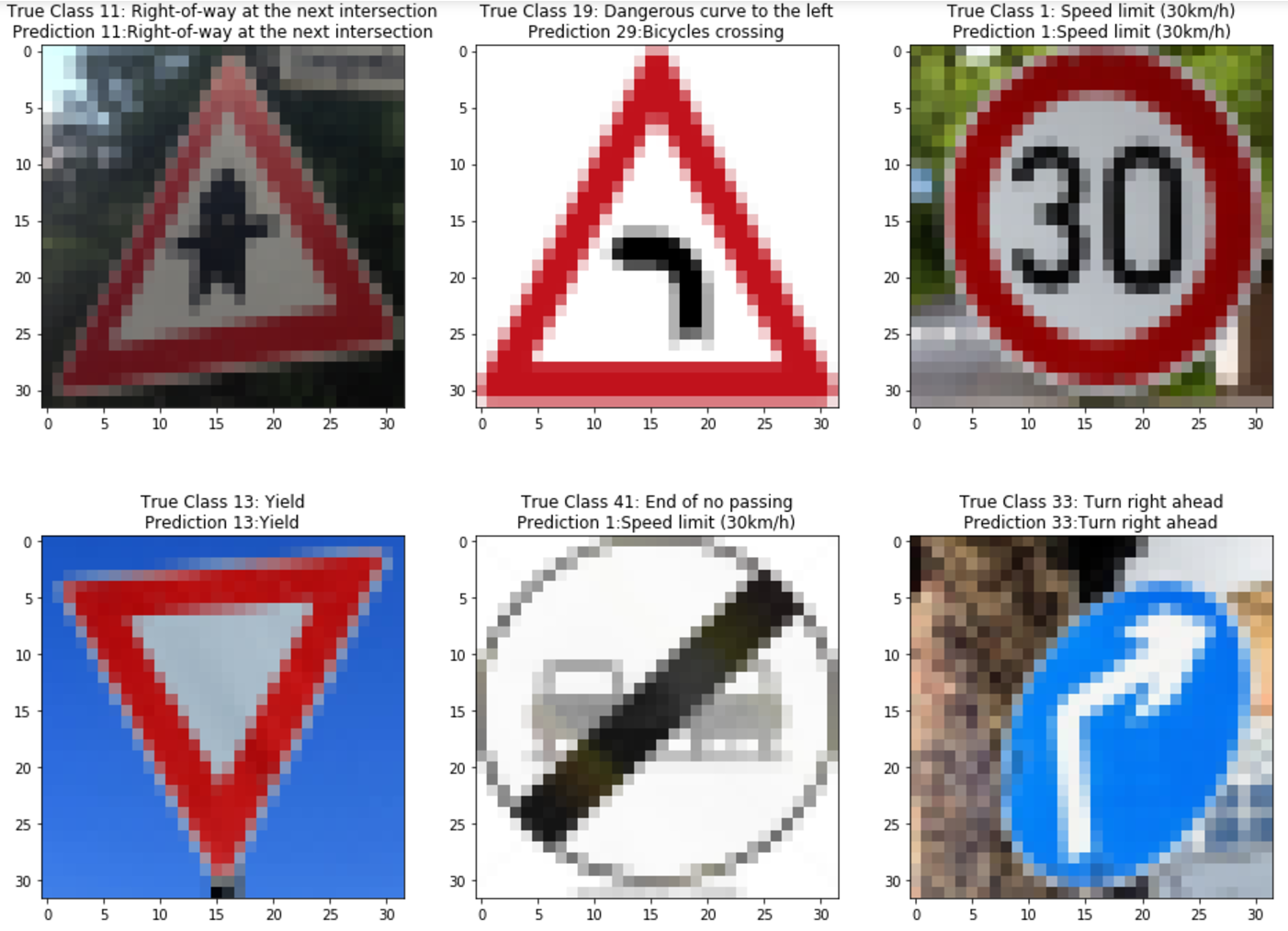
Six test images were downloaded from the internet to test my model as shown below. All of the six images are relatively easy to be recognized, since they are in overall clearly taken. Although the first (true class id 11) and sixth (true class id 33) are not in the front view, but this have been incoorporated in the augmented data by applying affine transform. The prediction on the second (true class id 19) and fifth (true class id 41) are incorrect. This may be explained by the asymmetry of the augmented data, since the proportion of Class 19 and Class 41 are low. It may be inapproprate to keep the proportion of classes in the augmented data. My improvement will be training the model with symmetric augmented data.

The top five softmax probabilities for each test image by my model are listed below. It seems my model is very confident on its prediction. For correctly predicted images, the model is 100% sure on the best choice. Although probabilities of the best predictions are not 100% for incorrect predictions, the probabilities are greater than 99%. Referred to images of each class shown above, the top 5 predictions for incorrect predictions are very similar to the truth, e.g. red triangular frames are observed for all top 5 preditions for Image 3. Differences between those predictions exist in the center of the red triangle frame. In order to recognize these small scale differences, multiscale structures may be considered to improve my model.

Image 1: Right-of-way at the next intersection

Probability	Prediction
100%	Right-of-way at the next intersection
0%	Pedestrians
0%	General caution
0%	Beware of ice/snow
0%	Ahead only

Image 2: Dangerous curve to the left

Probability	Prediction
99.92%	Bicycles crossing
0.08%	Road narrows on the right
0%	Dangerous curve to the left
0%	Road work
0%	Pedestrians

Image 3: Speed limit (30km/h)

Probability	Prediction
100%	Speed limit (30km/h)
0%	Speed limit (20km/h)
0%	Speed limit (50km/h)
0%	Speed limit (70km/h)
0%	Speed limit (80km/h)

Image 4: Yield

Probability	Prediction
100%	Yield
0%	Speed limit (120km/h)
0%	Beware of ice/snow
0%	Keep right
0%	General caution

Image 5: End of no passing

Probability	Prediction
99.8%	Speed limit (30km/h)
0.13%	Road work (120km/h)
0.06%	End of no passing
0%	Priority road
0%	End of no passing by vehicles over 3.5 metric tons

Image 6: Turn right ahead

Probability	Prediction
100%	Turn right ahead
0%	Ahead only
0%	Go straight or right
0%	Keep right
0%	Roundabout mandatory

For the second image ...

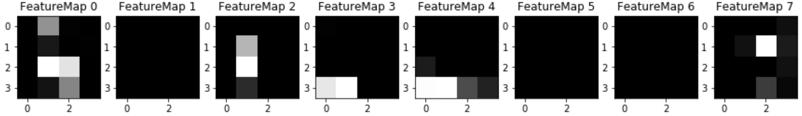
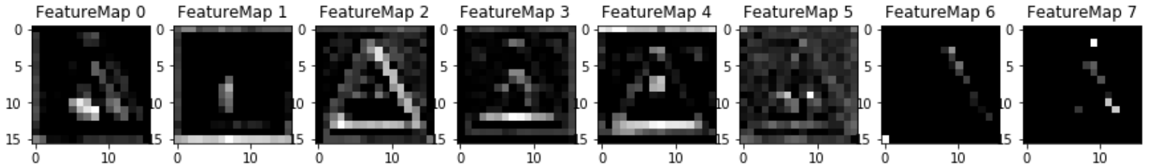
(Optional) Visualizing the Neural Network

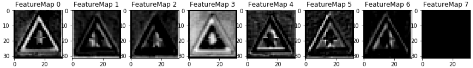
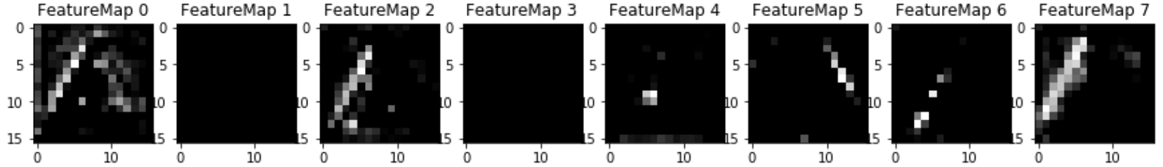
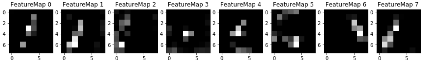
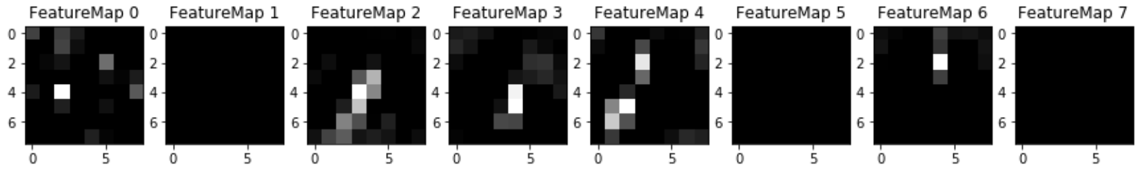
Eight arbitrary feature maps from the outputs of each convolutional layers are shown below. The observation is that the inner network feature maps react with high activation to the sign's boundary outline or to the contrast in the sign's painted symbol.